Note: This article was originally published on Hockey-Graphs 2019-01-14
Introduction
In this piece we will cover Adjusted Plus-Minus (APM) / Regularized Adjusted Plus-Minus (RAPM) as a method for evaluating skaters in the NHL. Some of you may be familiar with this process – both of these methods were developed for evaluating players in the NBA and have since been modified to do the same for skaters in the NHL. We first need to acknowledge the work of Brian Macdonald. He proposed how the NBA RAPM models could be applied for skater evaluation in hockey in three papers on the subject: paper 1, paper 2, and paper 3. We highly encourage you to read these papers as they were instrumental in our own development of the RAPM method.
While the APM/RAPM method is established in the NBA and to a much lesser extent the NHL, we feel (especially for hockey) revisiting the history, process, and implementation of the RAPM technique is overdue. This method has become the go-to public framework for evaluating a given player’s value within the NBA. There are multiple versions of the framework, which we can collectively call “regression analysis”, but APM was the original method developed. The goal of this type of analysis (APM/RAPM) is to isolate a given player’s contribution while on the ice independent of all factors that we can account for. Put simply, this allows us to better measure the individual performance of a given player in an environment where many factors can impact their raw results. We will start with the history of the technique, move on to a demonstration of how linear regression works for this purpose, and finally cover how we apply this to measuring skater performance in the NHL.
History
Adjusted Plus Minus (APM) was first developed publicly for the NBA in 2004 by Dan Rosenbaum here. Rosenbaum originally used a multiple linear regression (ordinary least squares regression) with points margin per 100 possessions as the target variable (dependent variable) and each player as predictor variables (independent variables). The data is grouped into observations separated by a “shift” of play where no player substitutions occur. This looks like a large data table with one row for each shift, and one column for each player who played within the respective season (or respective time period if multiple seasons are used). The columns for each player are categorical variables that are assigned values of 1, 0, or -1: 1 if they were on the court for an offensive shift, 0 if they were not on the court for a shift (or not in the specific game), and -1 if they were on the court for a defensive shift. The regression is run and the resulting coefficients for each player are collected. These coefficients are interpreted as each player’s individual contribution to the league point margin per 100 possessions with all other predictor variables held constant.
This technique was taken further in 2008 by Steve Ilardi and Aaron Barzilai [here] when they developed a method that allowed for two variables to be created for each player – one for offense and one for defense. Using this technique, each shift is duplicated and a 1 or 0 is assigned to the respective variables if a player was on the ice for offense or defense. This regression returns two coefficients for each player – offense and defense ratings – where a positive offensive coefficient is “better” and a negative defensive coefficient is “better”. These ratings are combined to arrive at the final adjusted plus-minus figure.
The next innovation in this method was proposed by Joseph Sill in 2010 [here] where he applied a regularization technique to the standard OLS regression – in this case, ridge regression (or Tikhonov regularization). This introduces bias into the coefficient estimates to reduce the overall variance of the model. The main purpose of regularization is an attempt to handle the “multicollinearity” that exists between players who play a significant amount of time together.
It is the latter of the two techniques (separate offensive and defensive variables [Ilardi/Barzilai] + ridge regression [Sill]) that Brian Macdonald modified and developed for the NHL. Dawson Sprigings employed this method in his “Corsi Plus-Minus” model [here], and Domenic Galamini Jr. used this method for the shot generation/suppression portion of his HERO charts [here]. In addition to even-strength or 5v5 play, MacDonald took the standard RAPM model further and developed a method for powerplay/shorthanded situations. It is his work that we have based most of our RAPM regressions on.
As noted, APM/RAPM is not the only regression-based model that has been developed for the NHL. Here are additional regression techniques that have been developed to evaluate NHL players:
- A.C. Thomas, Samuel L. Ventura, Shane Jensen, and Stephen Ma’s “Competing Process Hazard Function Models for Player Ratings in Ice Hockey” model uses a similar design but different technique [here].
- Robert B. Gramacy, Shane T. Jensen, and Matt Taddy’s “Estimating Player Contribution in Hockey with Regularized Logistic Regression” uses logistic regression to evaluate NHL skaters [here].
- Emmanuel Perry’s WAR model available on http://corsica.hockey uses multiple regression techniques for evaluating NHL skaters [here].
- Micah Blake McCurdy’s Magnus Prediction Models available on https://hockeyviz.com also uses multiple regression techniques for evaluating NHL skaters [here].
Linear Regression Example / Overview
Before getting into the methodology of RAPM for hockey, it is important to explain how linear regression works – specifically how the coefficients from a linear regression are interpreted (as these are the player ratings that are produced from this model). While the RAPM method does not employ ordinary least squares regression (OLS, or what is often referred to as “linear regression”), the technique is quite similar. We are going to use a completely different problem to demonstrate this as we feel a smaller/simpler dataset allows for a better explanation. Please keep in mind that the following example is presented with our main goal in mind: evaluating skaters in the NHL. This simpler dataset has to do with fuel economy in cars. This may feel like a bit of stretch, but it’s not – OLS can deal with both problems the exact same way.
For this demonstration, we’re going to use the “FuelEconomy” dataset from Max Kuhn and Kjell Johnson’s Applied Predictive Modeling data which is available as a package in R. The first step is to get acquainted with the data. This dataset is a table that contains 1442 rows and 14 columns. Each row is a specific type of car (manufactured between 2010 and 2012), and each column is a specific attribute of each respective car. The purpose of this dataset is to build a statistical model to predict fuel economy (measured in miles per gallon) using the additional variables (columns) that are provided. Fuel Economy is a “continuous” variable meaning it is a variable that has a changing value or, to put it in different terms, continuous variables could have infinite possible values. Fuel Economy in this dataset ranges from 17.50 to 69.64 miles per gallon. Most of the variables provided, however, are categorical which means they are variables that fall into a particular category. For the purpose of this demonstration we will be focusing on five variables to predict Fuel Economy.
Here is the target variable (also known as the dependent variable):

Here are the predictor variables (also known as independent variables):

And here are the first 10 rows of the data for reference (arranged highest to lowest by Fuel Economy):

There are multiple terms for the dependent variable and independent variables. We choose to use “target variable” and “predictor variables” when describing this process as it is the most sensible in our minds. Please have a look [here] for more synonyms for these concepts.
In addition, there are many purposes for using linear regression – one is to build a model that can “predict” a desired target variable given future (unseen) data. Another is to try and understand the relationship(s) between the predictor variable(s) and the target variable. When using linear regression in the latter manner, the target variable and predictor variables may be called the “response” and “explanatory” variables, respectively. Because we feel it is confusing to have multiple names for the same thing, we will be sticking with “target” and “predictor” variables. Regardless, it is important to note that the purpose of a RAPM regression is not to predict future outcomes but, rather, to understand the relationships between the predictor variables and the target variable (the predictor variables in a RAPM regression are the players in a given sport).

With that laid out, let’s explore the data – specifically how the target and predictor variables are related to each other. Here is a correlation matrix plot to assist: Right away we see that EngDispl and NumCyl are negatively correlated with our target variable (FE). Additionally, we can see that EngDispl and NumCyl are highly correlated with each other. We won’t get into the issues that multicollinearity in a dataset can cause right now, but keep this in the back of your mind as it is something we’ll talk about later.
Now that we have a basic idea of what the data looks like, let’s run a linear regression in R. Remember, we are trying to “predict” Fuel Economy using the predictor variables listed above. The formula that we run looks like this (where “FE” is the target variable, everything after the “~” are the predictor variables, and the “data” is the data table used):
lm(
  FE ~ EngDispl + NumGears + NumCyl + DriveDesc + CarlineClassDesc,
  data = cars_data
  )
The lm() function in R handles the multi-level categorical variables for us (which means “dropping” one of the specific types within a specific category). The summary of the model is returned as such (modified for readability purposes):


What we see here are the coefficient estimates that are returned from the linear regression as well as the standard errors, t values, p values, and information relating to how well the model fits the data. You can see that EngDispl is a single variable (since it is continuous), and the categorical variables have been broken down into separate coefficients. Each of the categorical variables have been turned into what are called “dummy variables” – meaning additional columns have been created for each specific type within each specific categorical variable within the dataset. For instance, the NumCyl variable is always either 4, 5, 6, 8, 10, or 12 – in this case, five new “dummy” variables are created. Because we have six categories for this variable, one of the levels is “dropped” to provide a “reference”. The reason this is done is that including all six types within this category as dummy variables would create perfect collinearity between these six columns (linear regression cannot deal with this).
For each of the new columns that are created, if the specific car (row) is a 5-cylinder car the NumCyl5 column will be marked with a 1 and all of the other NymCyl columns will be marked with a 0. If the car is a 10-cylinder car, the NumCyl10 column will be marked with a 1 and all other NumCyl columns will be marked with a 0 and so on. This is the same for the other three categorical variables (NumGears, DriveDesc, and CarlineClassDesc), which is why we see so many variables in the model output above.
With that covered, let’s focus on the “Estimates” that are returned – specifically, what are they and what do they mean. To explain, we will quote Jim Frost from his explainer [here]:
“The coefficient [estimate] value signifies how much the mean of the dependent variable [target variable] changes given a one-unit shift in the independent variable [predictor variable] while holding other variables in the model constant. This property of holding the other variables constant is crucial because it allows you to assess the effect of each variable in isolation from the others.”
Knowing that, we can say that an increase in Engine Displacement by 1 liter decreases the mean of the target variable by 1.889 miles per gallon. If the car is a Compact Car, it increases the mean of the target variable by 4.226 miles per gallon. If a car is a 12-cylinder car, it decreases the mean of the target variable by 10.741 miles per gallon, etc. All of this is true with the other respective variables held constant. This is the fundamental aspect of linear regression that allows us to isolate each predictor variable and determine the overall impact each has on the target variable.
Note: technically each categorical variable in the model output above should be interpreted relative to the “dropped” or “reference” variable within the specific category.
The lm() output also gives us the standard error for each coefficient – meaning, one standard deviation above/below the coefficient estimate. So, using Engine Displacement again, we can say an increase in Engine Displacement by 1 liter decreases the mean of the target variable by 1.889 miles per gallon +/- 0.22 (the traditional 95% confidence interval would be 0.22 * 2 or +/- 0.44). We won’t cover the additional information provided in the model output (t values, p values, R^2, etc.), but if you are interested in what those concepts are please have a look here.
Lastly, as noted above, the lm() function handles the categorical/factor variables for us; however, in certain cases it is not possible to use the lm() function to deal with this type of variable. In that case, we can construct the design matrix manually (creating dummy variables [1 or 0] ourselves) and feed the lm() function the specific formula. In this case, the lm() function call in R would look like this:
lm(
  FE ~ EngDispl + NumGears.4 + NumGears.5 + NumGears.6 + NumGears.7 + NumGears.8 +
  NumCyl.5 + NumCyl.6 + NumCyl.8 + NumCyl.10 + NumCyl.12 + FourWheelDrive +
  TwoWheelDriveFront + TwoWheelDriveRear + 2Seaters + CompactCars + LargeCars +
  MidsizeCars + MinicompactCars + SmallPickupTrucks2WD + SmallPickupTrucks4WD +
  SmallStationWagons + SpecialPurposeVehicleminivan2WD + SpecialPurposeVehicleSUV2WD +
  SpecialPurposeVehicleSUV4WD + StandardPickupTrucks2WD + StandardPickupTrucks4WD +
  SubcompactCars + VansCargoTypes + VansPassengerType,
  data = cars_data_dummy
  )
And the dataset would look like this (partial view):

Adjusted Plus-Minus / Regularized Adjusted-Plus Minus
At this point you may be wondering – how does all of this relate to measuring the performance of hockey players? Well, imagine the exact same process we used above with a different dataset. Before, each row in the data was a specific car. Now each row is a specific “shift” in a hockey game where a “shift” is defined as a period of time in a game where no player substitutions are made. Before, the target variable was Fuel Economy in miles per gallon. Now the target variable is Corsi For per 60 minutes (shot attempts per 60 minutes) within each specific shift. Before, the predictor variables were Number of Cylinders, Number of Gears, Engine Displacement, etc. Now, the predictor variables are the score state of each shift (categorical), the strength state of each shift (categorical), if a faceoff occurred in the offensive or defensive zone (categorical), if a team was on the second night of a back-to-back (categorical), and each skater that was on the ice for the specific shift (categorical). This is the basic layout of the original Adjusted Plus-Minus method (translated into hockey terms).
The categorical variable for each skater on the ice of a shift is somewhat different from the categorical variables we went over in the “Fuel Economy” example. In the previous case, each type within a specific category was present in a single row. For skaters on the ice, as you can probably guess, this variable is spread out over multiple columns – 12 to be exact (this is sometimes called a “multiple membership” variable). Regardless, the dummy variables are made the same way: a new column is created for each skater in the dataset (within those 12 skater columns) and their presence on the ice for a shift is marked with a 1 and their absence from the ice is marked with a 0.
We will use the method of creating two variables for each skater – when a skater was on the ice for offense and when they were on the ice for defense. In order to accomplish this, we need to augment our dataset quite substantially. We will duplicate each shift (row), which allows us to change the target variable from Corsi Differential per 60 (basketball’s APM used point margin per 100 possessions) to CF60 for the home team in each shift and CF60 for the away team in each shift. Additionally, instead of making a single column to indicate when each skater was on the ice, we will make two. In the “home team” shifts we mark the skaters on offense as “1” in their offensive variable column if they are playing for the home team and the skaters on defense as “1” in their defensive variable column if they are playing for the away team (all other skaters are marked with a “0”). In the “away team” shifts, this is reversed (away skaters are marked with a “1” in their respective offensive variable columns, home skaters are marked with a “1” in their respective defensive variable column and all other skater are marked with a “0”). Finally, we add a new binary categorical variable to denote if the shift is a “home team” or “away team” shift (“1” if the shift has the home team’s CF60 as the target variable and “0” if the shift has the away team’s CF60 as the target variable).
Here are the variables that we will use to run the RAPM regression:
Target variable:

Predictor variables:

We will be using the ‘17-18 season at even-strength (5v5, 4v4, and 3v3) for demonstration. The final dataset contains 586,018 rows (293,009 total shifts) and 1794 columns (1 target variable column, 1 weights column, and 1792 predictor variable columns). The mean length of each shift is 12.94 seconds and the mean CF60 is 62.12 (this is not comparable to the league mean CF60). Each skater who played more than 1 minute at even-strength in this season is included as a predictor variable (goalies are not included in the Corsi regression).
Here is a partial view of what this data looks like:

You will notice that the 5v5 strength state and the tied score state are not included – these have been dropped as references (same as we did above in the “Fuel Economy” example). None of the skater variables are dropped, but that will be covered a little later.
Now that we have a basic idea of the dataset, let’s move on to running the regression. The same principles apply from the “Fuel Economy” example but we need to make a couple modifications. First, because the target variable (CF60) is a rate (time dependent), we need to account for the length of each shift. This is handled using shift length (in seconds) as weights in the linear regression (this is traditionally called a “weighted least squares” regression). We won’t go into specifics, but this is similar to a weighted average – a longer shift has more “weight” in final model. We do this because we want to give more credit to a skater who maintains a high CF60 rate over the course of a long shift vs. a skater who maintains a high CF60 rate over a short shift.
Additionally, we will use a technique called “regularization” in the linear regression (this is where “Regularized” in “Regularized Adjusted Plus-Minus” comes from). Regularization in a linear regression comes in two main forms – ridge regularization (also known as Tikhonov regularization or L2 regularization) and LASSO regularization (“Least Absolute Shrinkage and Selection Operator”, also known as L1 regularization). The main purpose is to address multicollinearity that is present in the data. Why do we care about multicollinearity? Well, when a pair of players play together for a significant amount of time (the classic example is Henrik and Daniel Sedin who spent over 90% of their career time on ice together) the coefficient estimates in a traditional OLS regression will be extremely unstable (and therefore unreliable). Regularization combats this by adding some amount of “bias” into the model (Gaussian “white-noise”) to decrease the variance in the coefficient estimates [more info here]. What this means, essentially, is unstable coefficient estimates are “penalized” (or “shrunk”) based around a Gaussian distribution where 0 is the mean. Ridge regularization will pull coefficients towards 0 (but never exactly 0). LASSO regularization will pull coefficients toward 0 and also “zero” some coefficients. The LASSO is useful in certain models when “variable selection” is ideal; however, because we would like to obtain ratings for all skaters, we will use ridge regularization. Also, since skaters have separate coefficients (offense and defense), certain players will have only their offensive or defensive ratings zeroed which is not an acceptable outcome.
Note: ridge regression can also be interpreted in a Bayesian context – which is quite useful in this setting – but we’ll leave that for another article. This is covered in the above linked article (“more info”).
Let’s review. We are going to run a weighted ridge regression (regularized linear regression). The rows in the dataset are each shift in an NHL season separated by periods of play where no player substitutions are made. The target variable is the rate of shot attempts per 60 minutes (CF60) for the home team and the away team. The predictor variables are each skater on the ice for offense (home/away specific), each skater on the ice for defense (home/away specific), the score state (home/away specific), the strength state (universal), offensive/defensive “zone start” (home/away specific), back-to-back (home/away specific), and home team (if the target variable in the shift is CF60 for the home team). We will use R’s “glmnet” package to run this regression. The amount of “shrinkage” (penalization) of the coefficients is determined through cross validation. Luckily, glmnet will perform this for us. Here is the function call that is run in R:
cv.glmnet(
  x = RAPM_CF,
  y = CF60,
  weights = length_shift,
  alpha = 0,
  nfolds = 10,
  standardize = FALSE,
  parallel = TRUE
)
“RAPM_CF” is a table that contains all of the predictor variables (traditionally called the “design matrix”), “CF60” is a vector that contains the target variable for each shift, “length_shift” is a vector that contains the length of each shift (in seconds), “alpha = 0” specifies that we are using ridge regularization, and “nfolds = 10” specifies that we want to run “10-fold” cross validation to determine the lambda value (our shrinkage/penalty parameter) for the ridge regression (“standardize = FALSE” specifies that we do not want the function to standardize the predictor variables / “parallel = TRUE” specifies that we are using parallel processing to speed things up). This is a much different process than what we did with the lm() function earlier – this is because glmnet()/cv.glmnet() requires us to feed the design matrix (x), target variable (y), and weights separately.
This function returns an object that contains the lambda value that we will use for regularization – this is the amount of “shrinkage” (penalization) that will be applied. After cross validation is run, we are able to apply the regularization and extract the coefficients from the regression. Here are the non-skater predictor variable coefficient estimates:

Using what we know about linear regression, we can now see that being the home team increases the mean of the target variable (league average CF60) by ~2.4 CF60 (relative to being the away team with all other variables held constant). Additionally, we can see that a team on offense leading by 3 goals decreases the mean of the target variable (league average CF60) by ~9.02 CF60 (relative to the score being tied with all other variables held constant)… and so on. This is the beauty of using regression to evaluate hockey – inherently, linear regression provides estimates for each variable independent of the others.
Note: Unfortunately, because the coefficients in a regularized linear regression are “biased”, we cannot obtain the normal standard errors, t values, and p values that would be provided in a linear regression. Additionally, coefficients from a regularized linear regression do not represent the “true” change in the mean of target variable. They are “shrunk”/”penalized” and likely somewhat smaller than what the actual values should be (this is why they are not considered true unbiased estimators).
Next, let’s take a look at the skater coefficients. The below table has been restructured with each player’s offensive and defensive coefficients (labeled CF60 and CA60 respectively) on the same row. Each value is a separate coefficient from the regression that was run above (TOI, Team, Position were added for reference). Here are the top 20 highest rated players in “CPM60” which is the offensive coefficient minus the defensive coefficient from ‘17-18:

And the bottom 20 players:

Now, remember, since our target variable in this regression is CF60, the skater offensive and defensive coefficients are interpreted as each skater’s impact on the league average CF60 while on the ice for offense or defense respectively. Each skater variable is either a 1 or a 0 so the interpretation laid out above – a one-unit increase in the predictor variable – is interpreted as the skater’s presence on the ice. For instance, the presence of Mathieu Perreault on the ice increased the mean of the league CF60 by 6.90 while he was on offense and decreased the mean of the league CF60 by 3.16 when he was on defense (during the ‘17-18 season). This interpretation is the same for all skater variables that result from the regression.
Note: a negative value for defense is a good thing – a skater with a negative defensive coefficient decreased CF60 against while playing defense.
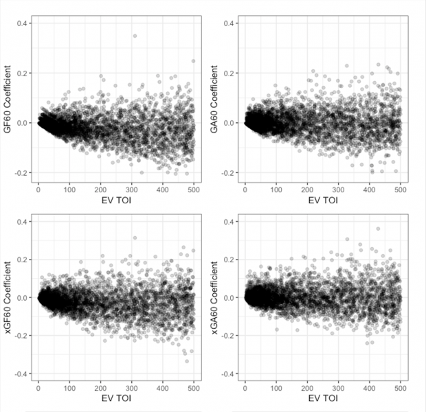
You may notice that all players shown in the above tables played somewhat significant minutes in ‘17-18 (even though all players with more than 1 EV minute played were included). This is the ridge regularization doing what it is intended to do. We can visualize this by plotting each player’s offensive and defensive coefficients against their respective time on ice at even-strength. The below chart includes each single-season regression from ‘07-08 through ‘17-18 filtered to players who played less than 500 minutes at even-strength for display purposes.

Note: This regression can be done for any metric – on https://evolving-hockey.com we provide regressions that use GF60 (goals for), xGF60 (our expected goals model [here]), and CF60 as the target variables. For the GF60 regression, we include goalies as defensive variables (it is assumed they have no impact on offense) – this is the original model that Brian Macdonald used. Additionally, for the GF60 and xGF60 variables, the score state variable is condensed from a 7-level factor (down by 3 goals through leading by 3 goals) to a 3-level factor (trailing/tied/leading).
Above, we can see that players who play less than ~100-150 EV minutes are being “regressed” to the mean (0 for each regression) – this is the regularization pulling these players towards the mean. Not only does this help to deal with multicollinearity (to an extent), it also adds a “quasi-Bayesian” aspect to the player ratings. In other words, if a player has very few shifts in the data, they are brought closer to the league mean using a Gaussian “prior” distribution. In an OLS regression, these players would have wildly inflated per 60 ratings.
So let’s summarize what the RAPM coefficients are. They are offensive and defensive ratings for each player that are isolated from the other skaters they played with, the other skaters they played against, the score state, the effects of playing at home or on the road, the effects of playing in back-to-back games, and the effects of being on the ice for a shift that had a faceoff in the offensive or defensive zone.
To get a better idea of what the RAPM ratings look like at even-strength, here are the distributions of the EV GF60, xGF60, and CF60 offensive and defensive ratings (single season ratings from ‘07-08 – ‘17-18, 150+ minutes):

Team Regularized Adjusted-Plus Minus
Skaters are not the only thing we can measure using a regression technique – we can also measure team performance. In this case, the setup is the same, but instead of using skater offensive and defensive variables we use team offensive and defensive variables. This is a much smaller dataset (rather than 1700+ skater predictor variables we have 60 team predictor variables – two for each team). This “Team RAPM” can be used to verify that the regression is doing what we want it to be doing (measuring the intended target variable “correctly”). To check this, we can plot the Team RAPM (per 60) coefficients against the Raw per 60 numbers. The below table shows Team Even-Strength RAPM regression results against the Raw per 60 results for each single season from ‘07-08 – ‘17-18:

The R^2 of each of the above plots is between 0.8 and 0.9 meaning the EV Team RAPMs explain around 80% – 90% of the variance in the raw per 60 results. The EV RAPM “team ratings” are, essentially, strength of schedule, score/venue, and back-to-back adjusted as well as adjusted for the seasonal environment – this most likely explains the differences we see above.
Powerplay/Shorthanded RAPMs
We’re not going to cover the PP/SH RAPM extensively, but it is worth explaining. Brian MacDonald introduced a Powerplay / Shorthanded RAPM model in the second paper he wrote on RAPM [here]. The powerplay/shorthanded model is very similar to the even-strength model; however, instead of creating two versions of each shift (to allow inclusion of offensive and defensive predictor variables for each skater), four versions of each shift are created containing the following target variables:
- Home Team CF60 while up a skater (5v4, etc.)
- Home Team CF60 while down a skater (4v5, etc.)
- Away Team CF60 while up a skater (5v4, etc.)
- Away Team CF60 while down a skater (4v5, etc.)
This allows us to create four predictor variables for each player which result in four player ratings:
- Powerplay Offense
- Powerplay Defense
- Shorthanded Offense
- Shorthanded Defense
Conclusion
Regularized Adjusted Plus-Minus is not a new concept in sports statistics, but it hasn’t caught on in public hockey work the way it has in basketball. We’ve implemented our own version of this method and tried to better demonstrate how it works and what it looks like in this article. We hope this provides greater transparency and helps others better understand the method. Additionally, the RAPM models are not limited to a given time frame either. They can be used to evaluate performance over any number of seasons, and it is often beneficial to use this technique over more than one season. For instance, we have 3-year RAPM models (covering the most recent 3-year timeframe) available on our site (https://www.evolving-hockey.com/). We also utilize a career-sum or long-term version in our WAR model – we cover how this works in more detail here (future links). Please let us know if you have any questions or suggestions in the comments below or on twitter (DMs are open @EvolvingWild), or via email (evolvingwild @ gmail . com).
Acknowledgements
We would like to thank:
- Domenic Galamini Jr. for all the help he provided along the way
- Brian Macdonald for his work adapting and developing the original RAPM method for hockey
- A.C. Thomas, Sam Ventura, Emmanuel Perry, Micah Blake McCurdy, and Dawson Sprigings for various prior work
—
Addendum
Here are the 20 top & bottom rated players for the EV single-season GF60, xGF60, and CF60 RAPMs:
Top 20: GF60 EV RAPM, ‘07-08 – ‘17-18

Bottom 20 : EV GF60 RAPM, ‘07-08 – ‘17-18

Top 20: EV xGF60 RAPM, ‘07-08 – ‘17-18

Bottom 20: EV xGF60 RAPM, ‘07-08 – ‘17-18

Top 20: EV CF60 RAPM, ‘07-08 – ‘17-18

Bottom 20: EV CF60 RAPM, ‘07-08 – ‘17-18

Distribution of Shift Length:
Even-Strength:

Powerplay/Shorthanded:

Thank you for reading!
Epic
Thank you very much for providing such detailed walkthroughs of your work. The entire evolving-hockey references page is one of the best resources available for anyone interested in public hockey analytics