Note: this article was originally published on RPubs.com 2018-06-07
Background
Expected Goals (xG) as a metric has become common-place in hockey analytics circles over the past few years. xG now sits neatly next to Corsi and Fenwick as a metric that is quite useful for both team and player evaluation. The models/metrics we’re familiar with today generally use multiple seasons of RTSS data (NHL play by play data) and often include over 20 variables as inputs. All of these models have their roots in work done over a decade ago. The earliest versions were often described as “shot quality” models, attempting to more or less “weight” shot attempts using the data that was available. The first version of this method appears to have been developed by Alan Ryder in 2004 here. Following this, he wrote about some of the issues with the (then new) RTSS data here, which then led to further work from Ken Kryzwicki here and here, and Michael Schuckers here and here. There are a few additional articles on Alan Ryder’s website here as well. These methods/approaches worked alongside the generally simpler concept of “weighted shots”, explained in Tom Tango’s write-up here.
Brian MacDonald developed an xG model here that expanded on this prior work. This model was never made completely public, and is (as far we’re aware) not currently available publicly. He presented this at the 2012 SLOAN conference, where he expanded on the article and provided some important references and notes. MacDonald’s model appears to have been one of the first in hockey that really caught on – or at least the idea. It introduced a larger audience to the concept of Expected Goals in hockey – more specifically, what is the probability that any given shot will result in a goal? Since MacDonald’s original method was proposed, there have been multiple models developed using various approaches and techniques.
Dawson Sprigings and Asmae Toumi developed an xG model in 2015 here that became very popular in the hockey analytics community. Sprigings and Toumi proposed a “shot-multiplier” variable that incorporated “shooting talent” in the model and showed that it was “a better predictor of future scoring than Corsi, Goals”. Emmanuel Perry’s first model followed, and was hosted on his website corsica, which brought the metric to an even larger audience. The main difference between Sprigings and Perry’s respective models was shooter talent, which was omitted from Perry’s. Corsica underwent a renovation in the summer of 2017, and the original xG model was replaced with a new model.
So far, each model described has used logistic regression to predict goal probability. Peter Tanner – creator of Moneypuck.com – employed gradient boosting (GBM) instead of logistic regression and added a “flurry adjustment” to offset excess value gained from rebound shots. Additionally, rather than using rebound and rush shot classifiers, he used prior event variables in his model. His use of a gradient boosting algorithm and prior event variables was something we drew heavily on when creating our own model. You can read more about his process here.
Cole Anderson and Matthew Barlowe ( (@CrowdScoutSprts and @matt_barlowe on twitter) also created xG models that use logistic regression. These are entirely open-source and can be found here and here. More recently, Harry Shomer (@36Hobbit) created a model similar to Moneypuck’s using gradient boosting here and further expanded on it here and especially here. Harry covers some interesting concepts with regards to shooting talent that we’ll touch on later.
Note: we’d like to thank Manny Perry for the code he’s made available on his GitHub. Because we’ve referenced his code to the degree we have, we’ve picked up a lot of his naming conventions. We’d also like to thank Peter Tanner, Matt Barlowe, Harry Shomer, and Manny Perry for their help with various issues we’ve run into when building the model. We’ve also learned a lot from all of the authors mentioned above, and we are very grateful to them as well.
Introduction to the New Model
Our motivation for creating a new xG model was primarily for our own purpose – it is difficult to integrate an existing xG model into the NHL’s RTSS data given the various differences in sourced data. We also had our own ideas about aspects of the xG concept that could be improved – specifically relating to strength states. Currently, all public models use all situations fenwick shots with strength state as a specific feature variable (a “categorical” variable). Given the significant differences in play styles and scoring rates between even-strength, powerplay offense, shorthanded offense, and empty net situations in hockey, it seemed like a good idea to build four separate models for each of these specific play states. In the initial stages of testing, we determined that there was a benefit to creating separate models for each of these four strength states. Additionally, we hoped to incorporate multiple models in an ensemble; however, the additional training time and size of the data made this impractical. Our final model consists of four separate models: even-strength (5v5, 4v4, 3v3), powerplay and man-advantage situations (5v4, 4v3, 5v3, 6v5, 6v4), shorthanded offense (4v5, 3v4, 3v5), and shots directed towards an empty net. We used an algorithm called “eXtreme Gradient Boosting” – better known as “XGBoost” – for all four of these models.
The Process
For the data, we’ll be using the NHL’s RTSS data, scraped using Manny Perry’s dryscrape functions. Recently, Manny made all of the RTSS data public on corsica – this is basically the same data we’re using (we’ve just acquired it via his scraper). Here’s what we get with the RTSS data:
##  [1] "game_id"             "event_index"         "season"
##  [4] "game_date"           "session"             "game_period"
##  [7] "game_seconds"        "event_type"          "event_description"
## [10] "event_detail"        "event_team"          "event_player_1"
## [13] "event_player_2"      "event_player_3"      "event_length"
## [16] "coords_x"            "coords_y"            "players_substituted"
## [19] "home_on_1"           "home_on_2"           "home_on_3"
## [22] "home_on_4"           "home_on_5"           "home_on_6"
## [25] "away_on_1"           "away_on_2"           "away_on_3"
## [28] "away_on_4"           "away_on_5"           "away_on_6"
## [31] "home_goalie"         "away_goalie"         "home_team"
## [34] "away_team"           "home_skaters"        "away_skaters"
## [37] "home_score"          "away_score"          "game_score_state"
## [40] "game_strength_state" "highlight_code"
This is set up as follows: each row in the dataset is a specific “event type” that lists all corresponding skaters who were on the ice as well as the length of the event, the coordinates of the event (if recorded), the strength state, score state, teams, etc. The event types the NHL tracks and records are:
##  [1] "PGSTR" "PSTR"  "ON"    "FAC"   "BLOCK" "OFF"   "SHOT"  "HIT"
##  [9] "STOP"  "MISS"  "GIVE"  "PENL"  "GOAL"  "PEND"  "TAKE"  "GEND"
For our purpose, the following event types will be used (all others are filtered out of the dataset):
## [1] "GOAL" "SHOT" "MISS" "BLOCK" "FAC" "HIT" "GIVE" "TAKE"Preparation
Now that we’ve covered what we’ll be working with, let’s move on to preparing the data and setting up the model. We want to include anything and everything that might help the model better identify how and why any given goal was scored. So we’ll need to convert, format, arrange, and organize the above data in a way that the model will be able to consistently work with. Additionally, there are a few things we need to correct in the RTSS data itself and a few additional variables we can add from the existing data that the NHL doesn’t explicitly provide but can be generated.
As a reminder, we’re splitting the strength states into four separate datasets to create four separate models. We chose to use seven full seasons for the EV and PP models (’10-11 through ’16-17), and 10 seasons for the SH and EN models (’07-08 through ’16-17). There are a couple reasons for this – the main reason being computational time to train the models. Seven seasons of EV data is a very large dataset and the training time is immense. We also found that adding older seasons did not improve the overall performance significantly (this is true for both the EV and PP models). Using 10 full seasons for the SH and EN models did improve the performance, which makes sense as short-handed and empty net shots occur much less frequently than EV or PP attempts.
Additionally, shots taken during the following situations were excluded:
- 6v3 strength state
- Penalty Shots
- Shootouts
We decided to exclude the above to improve the accuracy of measuring the most important situations for skater evaluation. The 6v3 state occurs so infrequently, we deemed this unnecessary (and potentially problematic due to a class imbalance) to include. Shots taken in the shootout or awarded as a penalty shot are entirely different and deserve their own model – this could be explored further in the future.
The Code
The code chunks we’ll be presenting below are taken from the functions found in our prep scripts here. We initially attempted to make this entirely reproducible within this write-up (display, R output, messages etc.), but it was not feasible. However, we still think its beneficial to go through each preparation function to demonstrate the process. Please feel free to reach out to us on twitter (@EvolvingWild) if you would like more detail and/or help.
Using the coordinates provided with the RTSS data, we can add shot distance and shot angle. We can also parse the description of the event and pull out the recorded distance and zone (offensive, defensive, or neutral) where the event occurred. The below distance and angle calculations are taken from Manny Perry’s GitHub. Since the distance and angle calculation assumes any shot was taken from 89 feet or less, we will identify “long shots” and correct the distance and angle. Additionally, we will correct the strength state and count of skaters for penalty shots.
# From fun.pbp_expand()
pbp_add <- sample_pbp %>%

  # Manny's functions removed

    mutate(pbp_distance = suppressWarnings(as.numeric(sub(".*Zone, *(.*?) * ft.*", "\\1", event_description))),
           event_distance = sqrt((89 - abs(coords_x))^2 + coords_y^2),
           event_angle = abs(atan(coords_y / (89 - abs(coords_x))) * (180 / pi)),
           event_zone = ifelse((grepl("off. zone", tolower(event_description)) == TRUE), "Off",
                               ifelse((grepl("neu. zone", tolower(event_description)) == TRUE), "Neu",
                                      ifelse((grepl("def. zone", tolower(event_description)) == TRUE), "Def",
                                             NA))),
           event_zone = ifelse(event_zone == "Def" & event_type == "BLOCK", "Off", event_zone),
           event_zone = ifelse(event_type %in% st.fenwick_events & event_zone == "Def" & pbp_distance <= 64,
                               "Off",
                               event_zone),

           # Update distance calc for long shots (and various mistakes)
           event_distance = ifelse(event_type %in% st.fenwick_events &
                                     pbp_distance > 89 &
                                     coords_x < 0 &
                                     event_detail != "Tip-In" &
                                     event_detail != "Wrap-around" &
                                     event_detail != "Deflected" &
                                     !(pbp_distance > 89 & event_zone == "Off"),
                                   sqrt((abs(coords_x) + 89)^2 + coords_y^2),

                                   ifelse(event_type %in% st.fenwick_events &
                                            pbp_distance > 89 &
                                            coords_x > 0 &
                                            event_detail != "Tip-In" &
                                            event_detail != "Wrap-around" &
                                            event_detail != "Deflected" &
                                            !(pbp_distance > 89 & event_zone == "Off"),
                                          sqrt((coords_x + 89)^2 + coords_y^2),
                                          event_distance)),

           event_angle = ifelse(event_type %in% st.fenwick_events &
                                  pbp_distance > 89 &
                                  coords_x < 0 &
                                  event_detail != "Tip-In" &
                                  event_detail != "Wrap-around" &
                                  event_detail != "Deflected" &
                                  !(pbp_distance > 89 & event_zone == "Off"),
                                abs(atan(coords_y / (abs(coords_x) + 89)) * (180 / pi)),

                                ifelse(event_type %in% st.fenwick_events &
                                         pbp_distance > 89 &
                                         coords_x > 0 &
                                         event_detail != "Tip-In" &
                                         event_detail != "Wrap-around" &
                                         event_detail != "Deflected" &
                                         !(pbp_distance > 89 & event_zone == "Off"),
                                       abs(atan(coords_y / (coords_x + 89)) * (180 / pi)),
                                       event_angle)),

           event_zone = ifelse(event_type %in% st.fenwick_events &
                                 event_zone == "Def" &
                                 pbp_distance <= 64, "Off", event_zone),

           # Update penalty shot strength states
           game_strength_state = ifelse((grepl("penalty shot", tolower(event_description)) == TRUE) &
                                          event_team == home_team, "Ev1",
                                        ifelse((grepl("penalty shot", tolower(event_description)) == TRUE) &
                                                 event_team == away_team, "1vE", game_strength_state)),

           home_skaters = ifelse((grepl("penalty shot", tolower(event_description)) == TRUE) &
                                   event_team == home_team, 1,
                                 ifelse((grepl("penalty shot", tolower(event_description)) == TRUE) &
                                          event_team == away_team, 0, home_skaters)),

           away_skaters = ifelse((grepl("penalty shot", tolower(event_description)) == TRUE) &
                                   event_team == home_team, 0,
                                 ifelse((grepl("penalty shot", tolower(event_description)) == TRUE) &
                                          event_team == away_team, 1, away_skaters))
           )
After adjusting the raw data for distance, angle, and zone, we perform a few indexing/temporary processes for later joins found in the fun.pbp_index() function. We’re not going to address this specific function or post the code in this writeup, but it’s important to keep all of the data more or less connected, which is what this function does. Next, we perform the final two steps to ready the data for modelling. The first function is the initial prep process, which wrangles the data a bit more and creates the initial prior event variables (referred to as “last”). The second part (somewhat primitively) one-hot encodes or “dummifies” the categorical variables for the model.
# From fun.pbp_prep()
pbp_prep_EV <- pbp_add %>%
      filter(event_type %in% c("FAC", "GOAL", "BLOCK", "SHOT", "MISS", "HIT", "TAKE", "GIVE"),
             game_period < 5,
             !(grepl("penalty shot", tolower(event_description))),
             !is.na(coords_x),
             !is.na(coords_y),
             !(coords_x == 0 & coords_y == 0 & event_type %in% st.corsi_events &
                 (pbp_distance != 90 & event_type %in% st.fenwick_events))
             ) %>%
      group_by(season, game_id, game_period) %>%
      arrange(event_index) %>%
      mutate(seconds_since_last = game_seconds - lag(game_seconds),
             event_type_last = lag(event_type),
             event_team_last = lag(event_team),
             event_strength_last = lag(game_strength_state),
             coords_x_last = lag(coords_x),
             coords_y_last = lag(coords_y)
             ) %>%
      ungroup() %>%
      arrange(season, game_id, event_index) %>%
      filter(event_type %in% st.fenwick_events,
             game_strength_state %in% st.even_strength,
             !is.na(coords_x_last),
             !is.na(coords_y_last)
             ) %>%
      # Create prior events
      mutate(same_team_last =     1 * (event_team == event_team_last),
             is_home =            1 * (event_team == home_team),
             score_state =        ifelse(is_home == 1, home_score - away_score, away_score - home_score),
             event_detail =       ifelse(is.na(event_detail), "Wrist", event_detail),
             distance_from_last = sqrt((coords_x - coords_x_last)^2 + (coords_y - coords_y_last)^2),
      rename(shot_distance = event_distance,
             shot_angle = event_angle
             ) %>%
      select(game_id, event_index, season, game_date, game_period, game_seconds,
             game_strength_state, game_score_state, score_state, is_home,
             event_player_1, home_goalie, away_goalie,
             home_score, away_score, home_team, away_team, home_skaters, away_skaters,
             event_description, event_team, event_type, event_detail,
             coords_x, coords_y, pbp_distance, shot_distance, shot_angle,
             event_team_last, same_team_last, event_strength_last, event_type_last,
             seconds_since_last, distance_from_last, coords_x_last, coords_y_last,
             shift_ID, shift_length
             ) %>%
      data.frame()


# From fun.model_prep()
model_prep <- data %>%
      mutate(is_goal = 1 * (event_type == "GOAL"),

             state_5v5 = 1 * (game_strength_state == "5v5"),
             state_4v4 = 1 * (game_strength_state == "4v4"),
             state_3v3 = 1 * (game_strength_state == "3v3"),

             score_down_4 = 1 * (score_state <= -4),
             score_down_3 = 1 * (score_state == -3),
             score_down_2 = 1 * (score_state == -2),
             score_down_1 = 1 * (score_state == -1),
             score_even   = 1 * (score_state ==  0),
             score_up_1   = 1 * (score_state ==  1),
             score_up_2   = 1 * (score_state ==  2),
             score_up_3   = 1 * (score_state ==  3),
             score_up_4   = 1 * (score_state >=  4),

             wrist_shot =     1 * (event_detail == "Wrist"),
             deflected_shot = 1 * (event_detail == "Deflected"),
             tip_shot =       1 * (event_detail == "Tip-In"),
             slap_shot =      1 * (event_detail == "Slap"),
             backhand_shot =  1 * (event_detail == "Backhand"),
             snap_shot =      1 * (event_detail == "Snap"),
             wrap_shot =      1 * (event_detail == "Wrap-around"),

             prior_shot_same =  1 * (event_type_last == "SHOT" & same_team_last == 1),
             prior_miss_same =  1 * (event_type_last == "MISS" & same_team_last == 1),
             prior_block_same = 1 * (event_type_last == "BLOCK" & same_team_last == 1),
             prior_shot_opp =   1 * (event_type_last == "SHOT" & same_team_last == 0),
             prior_miss_opp =   1 * (event_type_last == "MISS" & same_team_last == 0),
             prior_block_opp =  1 * (event_type_last == "BLOCK" & same_team_last == 0),

             prior_give_opp =  1 * (event_type_last == "GIVE" & same_team_last == 0),
             prior_give_same = 1 * (event_type_last == "GIVE" & same_team_last == 1),
             prior_take_opp =  1 * (event_type_last == "TAKE" & same_team_last == 0),
             prior_take_same = 1 * (event_type_last == "TAKE" & same_team_last == 1),
             prior_hit_opp =   1 * (event_type_last == "HIT" & same_team_last == 0),
             prior_hit_same =  1 * (event_type_last == "HIT" & same_team_last == 1),
             prior_face =      1 * (event_type_last == "FAC")
             ) %>%
      select(is_goal,
             shot_distance, shot_angle, is_home,
             state_5v5:state_3v3,
             score_down_4:score_up_4,
             game_seconds, game_period, coords_x, coords_y, coords_x_last, coords_y_last,
             wrist_shot:wrap_shot, distance_from_last, seconds_since_last,
             prior_shot_same:prior_face
             ) %>%
      data.matrix()
After completing these preparation functions, we have a dataframe that is ready to be prepared for modelling. We trained our models on the following fenwick shot totals for each of the four strength states.
| Strength State | Total Fenwick Shots |
|---|---|
| Even Strength | 537,519 |
| PP / Man Advantage | 113,573 |
| Shorthanded Offense | 23,714 |
| Empty Net | 3,680 |
And for reference, here are the total number of fenwick shots that were missing coordinates for the shot or prior event:
| Season | Percentage |
|---|---|
| 2017 – 2018 | 0.0128 |
| 2016 – 2017 | 0.0167 |
| 2015 – 2016 | 0.0118 |
| 2014 – 2015 | 0.0196 |
| 2013 – 2014 | 0.0180 |
| 2012 – 2013 | 0.0154 |
| 2011 – 2012 | 0.0185 |
| 2010 – 2011 | 0.0155 |
| 2009 – 2010 | 0.0198 |
| 2008 – 2009 | 0.0188 |
| 2007 – 2008 | 0.0284 |
Finally, we need to prepare the data for use with the xgboost package:
# Make sparse
model_data_sparse <- Matrix(model_prep_EV, sparse = TRUE)

# Separate into target / predictors
is_goal_vect <- model_data_sparse[, 1]
predictors_matrix <- model_data_sparse[, 2:ncol(model_data_sparse)]

# Full XGB data model
full_xgb <- xgb.DMatrix(data = predictors_matrix, label = is_goal_vect)
Given the amount of observations and the types of variables we’re working with, we converted all the data to sparse form with the Matrix function above (this essentially removes any 0 from memory). We then separated the target variable (is_goal_vect) and the features/predictors (predictors_matrix) into different objects to create a xgb.DMatrix object – this not only allows for easier use in modelling but gives one access to additional features within the package. The “predictors_matrix” above includes all the features that will be included in the final model. The features that were used in training the model(s) are listed below. We’ve separated them into continuous and Boolean (categorical) groups for display.
Continuous Variable
    shot_distance
    shot_angle
    game_seconds
    game_period
    coords_x, coords_y
    coords_x_last, coords_y_last
    distance_from_last, seconds_since_last
Boolean / Dummy Variables
    is_home
    state_5v5, state_4v4, state_3v3
    score_down_4, score_down_3, score_down_2, score_down_1
    score_up_4, score_up_3, score_up_2, score_up_1
    score_even
    wrist_shot, deflected_shot, tip_shot, slap_shot, backhand_shot, snap_shot, wrap_shot
    prior_shot_same, prior_miss_same, prior_block_same, prior_give_same, prior_take_same, prior_hit_same
    prior_shot_opp, prior_miss_opp, prior_block_opp, prior_give_opp, prior_take_opp, prior_hit_opp, prior_face
You may notice that we’ve yet to discuss shooting talent, which is also not present as a feature here. We’ll go into more detail about this subject at the end. Additionally, the Boolean features can really be summed for each line (is_home, strength state, score, shot type, etc). Because of this we think it’s more accurate to say we’ve used 15 features here instead of the 43 that are shown. Technically we’re using 43, but the 8 groups of dummy variables are intrinsically connected.
Modelling
Expected Goals as a model is a binary classification problem where the response/target variable is either a 1 or a 0 (1: a fenwick shot resulted in a goal // 0: a fenwick shot was not a goal). Only unblocked shots will be included (as the coordinates for blocked shots are recorded based on where the shot was blocked – not where it was taken). As we mentioned earlier, we’ve decided to use a form of gradient boosting called eXtreme Gradient Boosting, or XGBoost. Please reference the following articles for additional information if you’re interested in learning more: the R documentation, boosted trees overview, a gentle introduction to XGBoost, a more in depth overview of the algorithm, and the Leo Breiman and the Jerome Friedman journal articles that more or less developed the theories behind GBM.
This model is relatively simple on an abstract level, but the algorithm and package can be quite confusing if you’re new to it. The xgboost package in R offers an incredible amount of tuning parameters (called “hyperparameters”). We’ll generalize a bit here for the sake of demonstration: Logistic Regression has zero tuning parameters, Support Vector Machines has 1-2 (plus specific kernel parameters), and XGBoost offers well over 50 different parameters. It can be daunting. We used a “modified” random search method to tune to hyperparameters (demonstrated below). Given the extremely large data set, a true “grid search” method was simply not possible.
The following is the entire process we used to tune and trim the parameters with the xgb.cv function. As you’ll see, we used 5-fold cross validation run in a loop 200 times. Ultimately, our goal was to find the best set of parameters given our evaluation metric and the computational time – the latter being a much bigger influence than both of us had initially realized. The approach we chose took ~16 hours to complete for the EV model. Additionally, we ran this process for EV ~8 times. We included both Log Loss and Area Under Curve (AUC) as evaluation metrics. AUC was used to train and tune the final model parameters – Log Loss was included to reference. To demonstrate, the following process was used to train the even-strength model (this process is the exact same for the other strength states).
### XGB cv loop - EV
run_num <- 5
#run_num <- 200
best_df <- data.frame(matrix(nrow = run_num, ncol = 10))
best_ll <- data.frame(matrix(nrow = run_num, ncol = 5))


# Loop
for (i in 1:run_num) {

  print(paste("### LOOP:", i, "###"))

  param <- list(objective = "binary:logistic",
                eval_metric = "logloss",
                eval_metric = "auc",

                #max_depth = sample(6:10, 1), # run 1
                #max_depth = sample(6:7, 1),  # run 2
                max.depth = 6,                # run 3

                #eta = runif(1, .01, .3),  # run 1
                #eta = runif(1, .05, .15), # run 2
                eta = runif(1, .06, .11),  # run 3
                #eta = .1,                 # misc

                #gamma = runif(1, 0.05, 0.15),  # run 1
                gamma = runif(1, 0.06, 0.12),   # run 2 / 3
                #gamma = 0,                     # misc
                #gamma = runif(1, 0.0, 0.2),    # misc


                #subsample = runif(1, .6, .9),   # run 1
                #subsample = runif(1, .75, .85), # run 2
                subsample = runif(1, .76, .84),  # run 3
                #subsample = .7,                 # misc

                #colsample_bytree = runif(1, .5, .8),  # run 1
                #colsample_bytree = runif(1, .75, .8), # run 2
                colsample_bytree = runif(1, .76, .8),  # run 3

                #min_child_weight = sample(1:40, 1), # run 1
                #min_child_weight = sample(5:35, 1), # run 2
                min_child_weight = sample(5:22, 1),  # run 3

                #max_delta_step = sample(1:10, 1)    # run 1
                max_delta_step = sample(4:8, 1)      # run 2 / run 3
                )

  # CV
  rm(.Random.seed, envir = globalenv())
  x <- round(runif(1) * 10000, 0)
  set.seed(x)

  cv_param <- xgb.cv(data = full_xgb,
                     params = param,
                     nthread = 4,
                     nfold = 5,
                     nrounds = 1000,
                     verbose = T,
                     early_stopping_rounds = 25
                     )

  # Record results
  best_df[i, ] <-  unlist(param)
  best_ll[i, 1] <- min(cv_param$evaluation_log$test_logloss_mean)
  best_ll[i, 2] <- which.min(cv_param$evaluation_log$test_logloss_mean)
  best_ll[i, 3] <- max(cv_param$evaluation_log$test_auc_mean)
  best_ll[i, 4] <- which.max(cv_param$evaluation_log$test_auc_mean)
  best_ll[i, 5] <- x
  }
This is then bound together once the loop is finished like so:
# Clean up and bind
colnames(best_df) <- names(param)
colnames(best_df)[2] <- c("eval_metric_1")
colnames(best_df)[3] <- c("eval_metric_2")
colnames(best_ll) <- c("ll", "ll_rounds", "auc", "auc_rounds", "seed")
best_all <- cbind(best_df, best_ll)
best_all <- na.omit(best_all)

# Arrange to get best run
best_all <- arrange(best_all, desc(auc))
We’ve condensed this into an easier viewing format, but picture this as a row within the above “best_all” dataframe:
# objective:        binary:logistic
# eval_metric_1:    loglss
# eval_metric_2:    auc
# max.depth:        6
# eta:              0.0820009
# gamma:            0.0624977
# subsample:        0.7788831
# colsample_bytree: 0.7815288
# min_child_weight: 9
# max_delta_step:   5
# ll:               0.18464
# ll_rounds:        178
# auc:              0.7824754
# auc_rounds:       168
# seed:             647
Note: At the time, we misunderstood what the “eta” paramter (learning rate) was, so it was also included as a tuning paramter. In Laurae++’s xgboost/lightgbm paramter site, she states “It is not a good practice to consider the learning rate as a hyperparameter to tune.” Luckily, the eta paramter mostly stayed in a useful range for every model, so it didn’t end up being a problem. Additionally, please refer to Laurae’s site for more information on all of the hyperparameters – it’s an incredible resource.
As you may have noticed, there are several commented-out lines within the “param” list created in the main CV loop. We left these in to better demonstrate our method (this is not a complete representation of every run, rather a few sets that were used). After each run (the 200-run CV loop), we’d get an idea of where the “best” runs were coming in for each parameter, which would allow us to bring the ranges for each parameter in bit by bit. By the last run, you can see that a few never changed (max_depth for instance stayed at 6), and the rest all moved closer to an ideal setting. There is potentially room for improvement, but we just didn’t have the computing power to do this another way given the 16-hour run time. Regardless, after ~6 good loops (>1000 total runs), we felt tuning was sufficient given the improvement in the evaluation metric(s).
The last step is to set the final hyperparameters and determine the number of rounds to be used to train the final model – the number of rounds is the total number of trees the model builds. The following parameters were the actual values used in our final EV model. We set the hyperparameters and created another loop to determine the best number of rounds and the seed to use for training. This took some time, but we found that the rounds/seed did change, often significantly. Given this, we felt it better to run this a few more times (20+). To summarize, the hyperparameters have been determined; we’ll hold those constant and run another CV loop to determine the number of rounds and seed. Once this is set, all that’s left is to train the model using the xgb.train function.
# Final parameters
param_7_EV <- list(objective = "binary:logistic",
                   eval_metric = "logloss",
                   eval_metric = "auc",
                   eta = .068,
                   gamma = .12,
                   subsample = .78,
                   max.depth = 6,
                   colsample_bytree = .76,
                   min_child_weight = 5,
                   max_delta_step = 5,
                   nthread = 4)

# CV rounds Loop
run_num <- 20
cv_test <- data.frame(matrix(nrow = run_num, ncol = 5))

for(i in c(1:run_num)) {

  print(paste("### LOOP:", i, "###"))

  rm(.Random.seed, envir = globalenv())
  x <- round(runif(1) * 10000, 0)
  set.seed(x)

  # Re-run cross validation with set parameters to determine number of rounds to train on
  cv_rounds <- xgb.cv(param = param_7_EV,
                      data = full_xgb,
                      nfold = 5,
                      nrounds = 1000,
                      verbose = 2,
                      early_stopping_rounds = 25,
                      prediction = T)

  # Record results
  cv_test[i, 1] <- which.max(cv_rounds$evaluation_log$test_auc_mean)
  cv_test[i, 2] <- max(cv_rounds$evaluation_log$test_auc_mean)
  cv_test[i, 3] <- which.min(cv_rounds$evaluation_log$test_logloss_mean)
  cv_test[i, 4] <- min(cv_rounds$evaluation_log$test_logloss_mean)
  cv_test[i, 5] <- x

  }

# Clean results and sort to find the number of rounds to use and seed
names(cv_test) <- c("AUC_rounds", "AUC", "LL_rounds", "LL", "seed")
cv_final <- cv_test %>%
  arrange(desc(AUC)) %>%
  add_row(AUC_rounds = mean(cv_test$AUC_rounds),
          AUC = mean(cv_test$AUC),
          LL_rounds = mean(cv_test$LL_rounds),
          LL = mean(cv_test$LL),
          seed = mean(cv_test$seed))


# Train the final model
set.seed(556)

xg_train_xgb <- xgb.train(data = full_xgb,
                          params = param_7_EV, # Determined and set above
                          nround = 189,
                          verbose = 2
                          )
With that, we have the complete EV xG model using XGBoost. We can now predict xG values for all applicable EV shot attempts for any season. The fun.pbp_full_add function in our preparation script will allow for this to be completed. This will add a column for every fenwick event that gives its corresponding xG value. As we’ve mentioned before, our intention is for this to be useful for anyone. Again, please reach out (@EvolvingWild on twitter) if you have any questions about implementing this!
Results, Discussion and Conclusion
As is customary, let’s run through some validation numbers and discuss model performance. This is a bit of tricky topic, in our opinion, as the dataset is so large and the way this has been discussed in the past has varied quite a bit. Recently, (and somewhat initially), the ROC Curve and AUC or Area Under Curve metric have been used to evaluate any given xG model’s performance. Dawson/Asmae went about this a different way with their model and used a new method to determine how well their xG model could predict future scoring (please see Part II in their article). Harry Shomer covered both of these methods along with a Log Loss measure in depth in his article as well. As mentiond earlier, we used AUC for our evaluation metric and have not currently performed a method like Dawson & Asmae/Harry – this could be explored in the future. Matt Barlowe and Cole Anderson also used AUC for their evaluation metric, and their results can be found in the articles linked in the introduction.
Below is a table showing the AUC and the Log Loss numbers for two evaluation sets. “CV” is our cross-validated test set results (these were produced after the parameters were set and the number of rounds were determined). “’1718” is how well we did in the ’17-18 season – because the model didn’t see this season (it was trained through the ’16-17 season), it also functions as a way to evaluate how the model performs. As with any model, even the best K-fold cross validated test set is often, to varying degrees, overfit. You can see that here – although short-handed offense somehow performed quite well in ’17-18 (given the limited number of shots in a single season).
| Strength | AUC – CV | AUC – ’1718 | LL – CV | LL – ’1718 |
|---|---|---|---|---|
| EV | 0.7822 | 0.7747 | 0.1847 | 0.1897 |
| PP | 0.7183 | 0.7018 | 0.2716 | 0.2817 |
| SH | 0.7975 | 0.8369 | 0.2148 | 0.2035 |
Neither of us are quite sure how to compare these results to that of others as most have given only a single number (AUC most of the time) without going into too much detail about where that number came from. This is mostly due to the different methods others have employed in building their respective models, the various forms of availability to the actual shot-event and corresponding xG values from each, or that some don’t exist anymore. Right now, we both feel comfortable saying the AUC and LL values fall somewhere between the CV and ’17-18 sets displayed above.
Features & Variable Importance
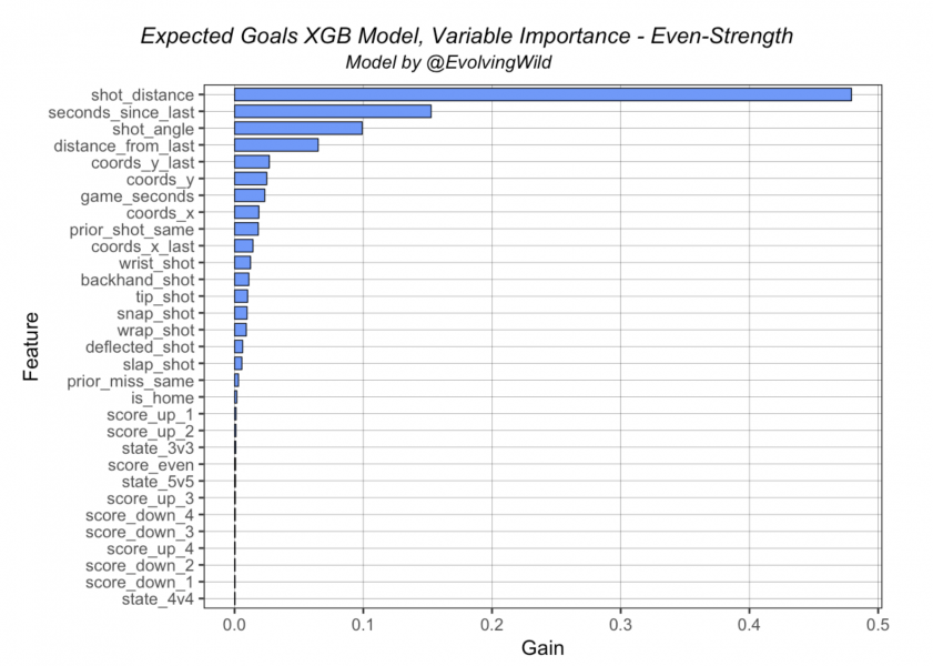
Even-Strength

Powerplay / Uneven-strength

Shorthanded Offense

Clearly, shot distance is the most “important” variable in the model, regardless of strength state. What this means, is that shot distance is the first “node” or split in the tree the vast majority of the time. Essentially, the algorithm splits any given shot into two groups up front based on the distance from the net of each shot. Variable importance charts are somewhat difficult to interpret with more advanced algorithms like XGBoost. While they’re very interesting to look at and do provide a view of the model that can give us some insight, it is important to note that these should not be interpreted in a manner similar to linear/logistic regression – these are not coefficients from a linear regression.
Shooting Talent
Let’s finally talk about “shooting talent”. This topic has been one of the more prominent debates/discussions surrounding xG models in hockey for the last several years. In Dawson/Asmae’s cited article, they included a shot multiplier as a variable to account for a given player’s shooting ability. This was calculated by regressing (adding a constant number of shots and goals to) a given player’s actual shots and goals. This produces a regressed shooting % for every player (regressed goals divided by regressed shots). Dividing this regressed shooting % by league average shooting % results in the “shot multiplier” that was used in their model. Given the amount of interest this approach generated at the time, we set out to create a similar variable that could be included in our own model. For this, we used a Bayesian method inspired by this fantastic article by David Robinson that explored a Bayesian technique for baseball batting averages. (We expanded on this this a bit in a tweet back in January ’18).
Both of us wanted to include a shooting talent variable; however, the algorithm did not feel the same. This variable (in each model) was never used in any decision tree that was generated – essentially, it determined that this variable added no value for predicting goals. Of course there’s the chance our method was flawed, which resulted in a less than ideal shooting talent variable for inclusion. Even so, we’re confident it wasn’t done so incorrectly as to be completely ignored. It makes intuitive sense that shooting talent should be included in xG, at least we think it does. We both have our theories about this, but this warrants additional research. Harry Shomer developd a very clever method where an initial xG model was built, and the xG values from that model were incorporated into a second model as a shooting talent variable here. He found that this increased the model’s performance. This is a method we would like to potentially explore in a future version of this model.
Examples & Final Thoughts
We also find that looking at specific shot events and their respective xG values can provide context for the models, what the features look like in practice/what the variable importance plots show, and help us to better understand how the models work. Here are the 5 EV shots with the highest xG value from the ’17-18 season predicted using our model:
| G | A1 | game_date | home | away | game_time | strength | type | pred_goal | Video |
|---|---|---|---|---|---|---|---|---|---|
| 1. ZEMGUS.GIRGENSONS | JACK.EICHEL | 2017-12-27 | NYI | BUF | 29.72 | 5v5 | GOAL | 0.9445601 | link |
| 2. MARC-EDOUARD.VLASIC | JOE.PAVELSKI | 2018-01-13 | S.J | ARI | 62.70 | 3v3 | GOAL | 0.9445432 | link |
| 3. JOHNNY.GAUDREAU | MATT.STAJAN | 2018-02-13 | BOS | CGY | 9.20 | 5v5 | GOAL | 0.9441528 | link |
| 4. ZACK.SMITH | DERICK.BRASSARD | 2018-02-21 | CHI | OTT | 15.93 | 5v5 | GOAL | 0.9440641 | link |
| 5. NICK.SHORE | -NA- | 2017-10-07 | S.J | L.A | 34.08 | 5v5 | GOAL | 0.9427717 | link |
As you can see, the shots with the highest probability of being a goal are those that are taken directly in front of the net that follow another shot. The model has identified this sequence as being an extremely high-danger situation. On the flip-side, here are the 3 shots with the highest xG value that did not result in a goal (again from the ’17-18 season):
| G | A1 | game_date | home | away | game_time | strength | type | pred_goal | Video |
|---|---|---|---|---|---|---|---|---|---|
| 1. MICHEAL.FERLAND | -NA- | 2017-11-30 | CGY | ARI | 28.58 | 5v5 | SHOT | 0.7356069 | link |
| 2. YANNI.GOURDE | -NA- | 2018-02-05 | EDM | T.B | 41.88 | 4v5 | SHOT | 0.7350974 | link |
| 3. KYLE.CONNOR | -NA- | 2018-01-30 | WPG | T.B | 51.60 | 5v4 | SHOT | 0.6556538 | link |
- 1. sequence from 3:55 – 4:20, shot at 4:04
- 2. sequence from 5:24 – 5:57, shot at 5:31
- 3. sequence from 6:39 – 6:54, shot at 6:51
Now, to demonstrate a few of the model’s potential weak points, let’s look at some goals that have attributes we don’t have access to (information that is not recorded by the NHL/not included in the RTSS data).
| G | A1 | game_date | home | away | game_time | strength | type | pred_goal | Video |
|---|---|---|---|---|---|---|---|---|---|
| VIKTOR.ARVIDSSON | FILIP.FORSBERG | 2018-03-01 | EDM | NSH | 39.83 | 5v5 | GOAL | 0.1712695 | link |
This was a classic 2-on-1 sequence with a clean cross-crease pass before the shot was taken. This event, while not necessarily “common”, is something we see somewhat often in the NHL. It is not surprising that this shot resulted in a goal. However, the model does not have access to any passing data (location or time of the pass) and doesn’t know where the players are on the ice (possibly player tracking data would allow this). The model only sees this as single shots taken close to the net.
Additionally, the following table shows a few more examples that demonstrate this point. The first two involve cross-crease passes that occur directly before the shot, and the third is a goal that followed a pass from behind the net. The xG values are all relatively low, however, these (intuitively) are very high-danger shots.
| G | A1 | game_date | home | away | game_time | strength | type | pred_goal | Video |
|---|---|---|---|---|---|---|---|---|---|
| ZACH.PARISE | MIKAEL.GRANLUND | 2016-01-05 | CBJ | MIN | 32.72 | 4v4 | GOAL | 0.1777228 | link |
| DAMON.SEVERSON | MARCUS.JOHANSSON | 2018-01-23 | BOS | N.J | 29.05 | 5v5 | GOAL | 0.06917952 | link |
| ALEX.CHIASSON | SAM.BENNETT | 2016-11-25 | BOS | CGY | 47.08 | 5v5 | GOAL | 0.08044741 | link |
Here’s another example of (our lack of and ability to capture) passing – the stretch pass. While these type of goals/shots are rarer, we believe this type of play would result in much higher xG value if passing data was available for us to use.
| G | A1 | game_date | home | away | game_time | strength | type | pred_goal | Video |
|---|---|---|---|---|---|---|---|---|---|
| KYLE.TURRIS | ERIK.KARLSSON | 2017-01-19 | CBJ | OTT | 16.28 | 5v5 | GOAL | 0.07192681 | link |
And just because we really enjoy looking at these, here’s an example of a good lo’ fashioned short-handed 2-0.
| G | A1 | game_date | home | away | game_time | strength | type | pred_goal | Video |
|---|---|---|---|---|---|---|---|---|---|
| TOMAS.PLEKANEC | MAX.PACIORETTY | 2014-10-25 | MTL | NYR | 12.1 | 4v5 | GOAL | 0.2327932 | link |
While we’d really like complete passing data, the above statements are mostly conjecture at this point. Both of us are fairly confident that any xG model would benefit somewhat significantly from knowing where a pass came from and when it occurred… and we haven’t even touched on zone entries/exits. A lot of this data is currently being tracked publicly, and this could be incorporated into future versions of xG models. Regardless, we feel the model still performs well given the data available.
Good stuff guys.