Note: this article was originally published on Hockey-Graphs 2019-01-06
In part 1, we covered WAR in hockey and baseball, discussed each field’s prior philosophies, and cemented the goals for our own WAR model. This part will be devoted to the process – how we assign value to players over multiple components to sum to a total value for any given player. We’ll cover the two main modeling aspects and how we adjust for overall team performance. Given our affinity for baseball’s philosophy and the overall influence it’s had on us, let’s first go back to baseball and look at how they do it, briefly.
Baseball WAR splits the various aspects of the game into components where each uses a different method to determine value. Each of the public models does this differently. For batting, however, they all for the most part use something called “linear weights”, which is a common name applied to the concept of adjusting RE24 – or “run expectancy based on the 24 base-out states” – to the league average for a given season. FanGraphs summarizes this concept nicely: “the average number of expected runs per inning given the current number of outs and placement of baserunners.” These numbers take the form of run expectancy tables or matrices (the below table is from the RE24 FanGraphs article):

These tables show the change in “run expectancy from the beginning of a player’s plate appearance to the end of it”. With these, the expected runs of a given offensive-event (a single, double, home run, etc) can be calculated relative to league average over a given length of time. This concept is then used in other metrics that form the higher-level structure(s) of some of the public WAR models – for instance, Tom Tango’s wOBA (weighted on base average) plays a major role in both Baseball-Reference’s and FanGraphs’ respective WAR models (and the overall framework of the public WAR models in baseball – he’s cited as the creator of this framework).
The public WAR models start to diverge on how they evaluate fielding (defense) and pitching, and while Baseball Prospectus uses the above concept of run expectancy for offense, their methods are quite a bit more advanced for every aspect of their WAR model. FanGraphs uses something called Ultimate Zone Rating (UZR), and baseball reference relies on something similar. Each of these, as well, takes prior expected run values for balls-in-play and assigns a value based on whether a defender, adjusted for position, converted that ball in play to an out (this is a crude explanation). What baseball has the luxury of is discrete “states”. To say it another way: there are only a certain number of outcomes, positions, bases, types of hits or ways to reach base. Baseball has structure in the ways that runs are scored (from a statistical perspective) – again this is simplistic.
Hockey, however, is not that simple. While a goal is scored (and with the RTSS data we have a lot information about each goal), evaluating how much credit a given player should receive for that goal is a much more difficult question. Obviously, hockey and baseball are different sports. Baseball has a certain built-in isolation for each event (hit, strike, out, home run, etc) – that’s why their linear weights approach works. The average value of all events can be determined by evaluating how those events have historically impacted run scoring. In hockey, this would be akin to binning locations on the ice, building a matrix in the spirit of the run expectancy matrices in baseball, averaging how often a goal resulted from a shot with a given position in the matrix historically, and applying these expected values to each type of event (shot, block, miss); or essentially an Expected Goals model. Problem solved!
Well, not really. Whether or not a player in baseball hit a double or triple, whether a pitcher recorded a strikeout or walk, these are largely isolated to just that given player’s performance. In hockey, goal scoring is a much more complex system of teammates and opponents and goalies and strength states etc. This is why we often use “on-ice” metrics to evaluate skaters. If a player scores a goal, it wasn’t just him that contributed to that goal, his teammates (and the defending skaters and the goalie) contributed to the goal as well among a host of other factors. We want to know how much all players are contributing to both offense and defense at all times, not just who actually scored.
We stated in part 1 that we set out to create a WAR model more in line with baseball, but it seems we’ve reached a pretty significant roadblock: the foundation for their models is not one that we can easily adapt for use in hockey evaluation. It seems baseball’s influence stops here. To be clear of what that influence is: “we want to know what a player has done” (BP). We aren’t concerned with whether this is repeatable or predictive of future results. Hence, our WAR model will attempt to assign value for what a player did in the best way we can. Say goodbye to baseball for now! It’s time to look at how another sport deals with these issues.
Basketball – A Different Approach
Basketball analysts have developed an incredible number of techniques for player evaluation that allow us to deal with a continuous sport like hockey where many moving pieces play a role in contributing to scoring and preventing scoring. We are lucky that a lot of this work and research is still available for us to use and adapt, which is what we’ve done. We haven’t talked much about modeling in baseball – and for the most part, that’s because the public baseball WAR models do not implement any kind of models in the statistical sense (linear regression, machine learning, etc.) – this excludes Baseball Prospectus, and also anything that we’re unfamiliar with, apologies. The work done for evaluating players in the NBA, however, has relied heavily on statistical modeling.
We covered what one of these methods looks like extensively in our Regularized Adjusted Plus Minus (RAPM) write-up a few days ago. Please give this a read if you haven’t yet because we won’t be covering the history or how it works here. What RAPM allows us to do is utilize a statistical technique that accounts for all players on the ice (including teammates and opponents), score state, zone starts, among other things. We use ridge regression (also known as Tikhonov Regularization or L2 regularization) to evaluate all skaters’ impact on the mean of a given dependent/target variable. In this case, we can use Corsi (shot-attempts), Expected Goals, or Goals as a target variable at a shift-by-shift level built using the NHL’s RTSS data, where each shift is separated by a period of play where no player substitutions are made. While we demonstrated RAPM using one season in the above article, the timeframe is not limited – any number of seasons can be included.
The methodology we’re using is directly influenced by the techniques used in basketball for NBA analysis: create individual player ratings using RAPM for a given timeframe, use those values for a separate model that uses RTSS-derived metrics (goals, relative to teammate metrics, zone start percentages, etc.) to create single season values (which we call Statistical Plus Minus or SPM), and convert the SPM output(s) to the eventual WAR components. In the case of RAPM’s use in our WAR model, we’re using long-term values and corresponding long-term RTSS-derived metrics for the SPM models. This covers the ’07-08 season through the end of the ’17-18 season (11 years). Now that we’ve laid this out, here is an overview of the entire process for our WAR model in a handy flowchart:

Note: for the long-term RAPM that is used as the target variable of the corresponding SPM models, we’ve standardized all predictor variables and used cross-validation to determine a TOI cutoff for players included in both models. This allows us to remove players from the dataset that have not played enough time in the NHL for us to reliably match a long-term RAPM to various RTSS-derived metrics. We cover this more in our RITSAC ’18 presentation (presentation and slides).
Statistical Plus-Minus (SPM)
With the long-term RAPM model in place, we are ready to move on to the next step of the process: Statistical Plus-Minus. We’ve discussed the various Plus-Minus models in our RAPM article linked above (this is much different from traditional plus-minus in the NHL), and while the nomenclature may be similar, it’s important that we separate RAPM from SPM. While the RAPM and SPM models give us similar outputs (a player rating for each player), the inputs for each are drastically different.
First, let’s talk about the name. “Statistical Plus-Minus” was developed by Dan Rosenbaum in 2004 here – this article is a must read for anyone looking to learn more about the Plus-Minus stats in basketball. Neil Paine laid out how SPM works in a more straight-ahead fashion here, which shows the basketball SPM formula:
lm(formula = plus_minus ~ mpg + p36 + tsa36 + tsasq + tpa36 + fta36 + ast36 + orb36 + drb36 + stl36 + blk36 + tov36 + pf36 +versatility + usgast, weights = minutes)
This is the R code for a weighted linear regression, but notice the “plus_minus ~” part – this is where we diverge from the RAPM model. The “plus-minus” metric above is a specific set of player values determined using one of the basketball career-sum or long-term plus-minus methods (APM/RAPM). In Paine’s SPM, it appears the original Adjusted Plus-Minus method was used. The idea here is to run a long-term regression model (RAPM), take the outputs (player coefficients or player ratings) of that model, use them as our target variable in a new regression, and collect corresponding box score or play-by-play derived metrics as new features/predictors in this new regression for the corresponding players. With both the long-term target variable and corresponding long-term play-by-play derived metrics in place, we can create a new model: Statistical Plus-Minus.
Likely the most well known version of this method is Basketball-Reference’s Box Plus/Minus metric. Daniel Myers’ write-up on BR was instrumental in the creation of our model. Not only does he lay out the process, he covers the history of the various plus-minus methods quite well. For more background on the development of these methods, please reference Myers’ summary of them here, this post from Myers on the APBR forum, and Neil Paine’s comparisons of them on the same forum. For even more reading, a Bayesian APM method can be found here, Joseph Sill’s RAPM paper here, and this in-depth review of APM and RAPM from Justin Jacobs here.
Basketball has numerous names and methods and models for all of these, so why did we choose to use the SPM name for this part of our process? We’ve chosen to focus on the RTSS-era, which covers 2007 to current day (in our case through the ’17-18 season). BPM is specifically designed to work with historical data, and in turn has a limit on the number of box-score metrics it can use to create its model. This is somewhat arbitrary, but often SPM has used non-historical metrics for its model, which is what we’re doing, so we went with that name.
With that said, why do we need both RAPM and SPM? These methods are not easy to set up or run, and they take a long time to fine-tune and finalize. Here are a few important reasons for this process:
- Within a single season, multicollinearity can still be an issue with the RAPM method. It is difficult to determine just how much this affects the player ratings, which may make it difficult to rely entirely on RAPM within a given season on its own.
- The SPM approach helps us mitigate the issue of multicollinearity by estimating a player’s value using multiple metrics that are less affected by this problem. Because of this, we’re able to use the SPM model to estimate a player’s value on a smaller level.
- This also allows a certain amount of interpretability since we’re using RTSS-derived metrics to create player ratings. We can look at which metrics in the SPM models are significant and investigate further why a player’s final number looks the way it does.
- Most importantly, this method allows us to properly balance the respective magnitudes of each component in our WAR model. When using RAPM in-season for various components, the player ratings that each produce are not comparable to one another – the amount of regularization (“shrinkage”) applied to these separate ratings are not equal because the coefficient estimates are biased. What this means is that we may or may not see an unacceptable difference in magnitude between all of the components (even-strength offense and powerplay offense, for instance). Using another modeling technique to estimate a long-term RAPM output allows us to “scale” the values more accurately, which better represents the actual magnitudes of the respective components.
Using the RAPM -> SPM method allows us to bridge the gap from long-term player evaluation to granular value-added measurements for players. This method also gives us the ability to separate and measure different components of the game more effectively without worrying too much about the issues that long-term methods present. While the tradeoff here is possibly accuracy, the combination of multiple components with respect to their various magnitudes can be handled in a more appropriate way. Simply, we feel this allows us to properly sum all components to arrive at a single number. However, this means we need to not only create RAPM models and derive corresponding values for all the pertinent strength states/components, we have to then create SPM models for those same strength-states as well.
SPM setup
The RAPM model gives us our target variable (per 60), but we need to organize and collect our RTSS-derived metrics (per 60) to create this model. Remember, the SPM feature variables will keep the same long-term (11 year) aspects that the RAPM models did, but they will be the long-term values for individual metrics (think CF60 or GF60 over 11 years for every player). We also need to separate out all of these metrics per component. For skaters the components are:
- Even-Strength Offense
- Even-Strength Defense
- Powerplay Offense
- Shorthanded-Defense
Each of these components is then separated out by position for skaters. With each of these defined, we can collect our RTSS-derived metrics for the SPM process and begin to create the component-specific models that will eventually be used to create our Goals Above Average metrics. These are all of the metrics we were able to derive from the NHL RTSS data for offense (both EV and PP). All metrics are rate versions (per 60) unless otherwise noted.
- TOI percentage, TOI per GP
- G, A1, A2, Points
- G_adj, A1_adj, A2_adj, Points_adj (where “adj” means adjusted for state)
- iSF, iFF, iCF, ixG, iCF_adj, ixG_adj
- GIVE offensive zone, GIVE neutral zone, GIVE defensive zone (o/n/d are the same below)
- GIVE, GIVE_adj
- TAKE_o, TAKE_n, TAKE_d
- TAKE, TAKE_adj
- iHF_o, iHF_n, iHF_d
- iHF, iHF_adj
- iHA_o, iHA_n, iHA_d
- iHA, iHA_adj
- OZS_perc, NZS_perc, DZS_perc
- FO_perc, r_FO_perc (regressed faceoff %)
- rel_TM_GF60, rel_TM_xGF60, rel_TM_SF60, rel_TM_FF60, rel_TM_CF60
- rel_TM_GF60_state, rel_TM_xGF60_state, rel_TM_SF60_state, rel_TM_FF60_state, rel_TM_CF60_state (state adjusted)
And here are all of the defensive metrics (EV and SH) derived from the RTSS data (the same naming conventions were used):
- TOI_perc, TOI_GP
- iBLK, iBLK_adj
- GIVE, GIVE_adj,
- GIVE_o, GIVE_n, GIVE_d
- TAKE, TAKE_adj,
- TAKE_o, TAKE_n, TAKE_d
- iHF, iHF_adj,
- iHF_o, iHF_n, iHF_d
- iHA, iHA_adj,
- iHA_o, iHA_n, iHA_d
- OZS_perc, NZS_perc, DZS_perc
- FO_perc, r_FO_perc
- rel_TM_SA60, rel_TM_FA60, rel_TM_CA60, rel_TM_xGA60
- rel_TM_SA60_state, rel_TM_FA60_state, rel_TM_CA60_state, rel_TM_xGA60_state
A couple notes here regarding all of the metrics. We’ve been extremely influenced by the work of Emmanuel Perry; hence we’ve borrowed a lot of our naming conventions from him. Additionally, most of the above metrics are the standard metrics available on corsica.hockey among others. However, we’ve updated the Relative to Teammate metrics for our model (these are the “rel_TM” metrics). We wrote a two-part article for Hockey Graphs back in February, 2018 (part 1, part 2) that revisited how this metric works (based on David Johnson’s work from his old hockeyanalysis.com site) and proposed a few ways this method could be updated. After all that work, we actually ended up taking this metric one step further. Given that the individual SPM models rely on these stats quite heavily, it’s important we quickly cover this.
Relative to Teammate Original Calculation:
Rel TM CF60 = Player’s on-ice CF60 – weighted average of all Teammates’ on-ice CF60 without Player (weighted by Player TOI% with Teammate)
Relative to Teammate New Cacluation:
Rel TM CF60 = Player CF60 – weighted average of all Teammates on-ice CF60 (weighted by Player TOI% with Teammate)
So briefly, the original Rel TM metric was based on the time all of a given player’s teammates played without that player. In testing this in preparation for our SPM models, we found that the metric actually correlates better with the RAPM outputs if instead of using this “without” number, we use the total number for a given player’s teammates (the right side of the above equations is changed). We’ll likely have a part 3 to add on to the Relative to Teammate HG series, but for the time being, it’s important to remember that the Rel TM metrics we’re using are not the standard versions found on various sites. This new Rel TM metric, however, is available on our website (www.evolving-hockey.com).
Model Selection
Historically, basketball has used linear regression to fit their various BPM-style models. We’ve had a lot of success using other algorithms in our hockey work, and we thought we’d try out some of these for this process. Given R’s wealth of options when it comes to Machine Learning algorithms and the various libraries/packages that give us access to them with relative ease, it seemed only natural. A side-note: we use R’s Caret package quite often, which is maintained by the great Max Kuhn, and we used it for training these models. Ok, so we have a bunch of big sounding tools at our disposal, a ton of intimidating machine learning algorithms available, and just enough computing power to try it all out! Great!
Except… linear regression works very well for this problem. We thought surely some of our favorite ML algorithms would perform well here (Gradient Boosting specifically), but we laboriously discovered that linear regression was extremely difficult to beat when tuned properly. Once we investigate the RAPM outputs, however, it makes quite a bit of sense why this would be: given that RAPM uses a linear-type method, the outputs are understandably quite normally distributed. Take a look at the long-term forward EV GF RAPM for example:

We did find, however, that several of linear regression’s cousins worked quite well, especially for the defensive metrics. After much testing, we arrived at the following five algorithms to build our SPM models:
- Linear Regression (OLS)
- Elastic Net Regression (glmnet package in R)
- Support Vector Machines (w/ linear kernel from kernlab)
- Cubist (Cubist package in R)
- Bagged Multiple Adaptive Regression Splines (bagged MARS, bagEarth package in R)
Additionally, we decided to use an “ensemble” of these algorithms to fit our SPM model (here’s wikipedia’s explanation). Given that we wanted to use our model for both long-term and in-season (read: small sample) analysis and evaluation, we found using a collection of various algorithms blended together allowed us to better fit the long-term RAPM outputs for the ultimate use in our WAR model. After much testing and tuning, we found that using three algorithms for each component was the best approach.
We could extend the number of algorithms we use to any number, and our ensembles could include any number of algorithms as well. The reason we’ve “limited” the number for each step is for simplicity, but it also takes a long time to train, tune, and test 24 separate algorithms (4 total components * 2 skater positions * 3 algorithms). The more algorithms we include, the longer this takes. We found this setup was a good balance of added predictive power (as in the SPM models predicting out-of-sample RAPM in an evaluation sense) -AND- relative simplicity (there’s a certain amount of diminishing returns with added algorithms that we felt was important to mitigate mostly for our sanity).
Feature Selection
We’ve outlined the total RTSS-derived metrics above, and with each of these component models we will whittle down the available metrics to those determined to be most significant/important for “predicting” the respective RAPM outputs (our target variable in the SPM process). Feature selection was performed through a lengthy cross-validation process. Each “tuning” iteration consisted of 300 cross-validation runs where a model was trained on 80% of the data and tested on the 20% of data that was held out. The results of these 300 runs were then averaged. This process was repeated, each time adjusting the features that were included in each algorithm until the best set of features was achieved based on the aggregated root-mean-square error for a given tuning iteration. This was done for all 5 of the algorithms for each of the individual components (EV Offense, SH Defense etc). In total, we allowed five algorithms to be used for the 8 component models, which means 40 total algorithms were trained and tuned using the above process. Of those 40 algorithms, we selected the three best for each component, which means 24 algorithms were used in total to create the eight SPM component models (remember 4 components, split by position).
The linear regression sub-model features were selected based on p-value tuning, and the other four sub-models used each algorithm’s built-in feature selection process (bagged MARS for instance has two parameters – “nprune” and “degree” – that are tuned based on the features it’s fed. Cubist uses “committees” and “neighbors”, and so forth). Of note: we did remove several metrics that never performed well in our testing up front prior to tuning (Points, the state-adjusted metrics, the adjusted G/A1/A2 metrics, etc.). Additionally, there were several features that were highly correlated with one another (rel TM CF/SF/FF/xGF for instance) – the less significant metrics in the correlated “groups” were omitted prior to running the above validation processes, and only one of rel TM CF/FF/SF was included in any given training process (given how correlated they are). After all of that was finished, we arrived at the final features that were used for each of the SPM component models. Below we’ve displayed the final metrics that were included in each SPM component ensemble model.
Here is the setup for the following tables: the furthest-left column contains all of the features that were provided within a specific SPM-component model, the remaining columns are the algorithms used for the given SPM component (F and D indicate positions), and an “x” indicates when a metric was used by the algorithm. The metrics included in each model for each component (the furthest-left column) are ranked by importance, the highest being most important and lowest being the least. All of the features included here are in per 60 or “rate” form since the RAPM outputs/values are in this form.


We’ve chosen not to display the variable importance numbers for each of the SPM models here for a reason. While variable importance for individual models can be quite interesting to look at, we feel it is misleading, hard to interpret (even though that’s what it’s supposed to be for), and not all that helpful in understanding how the algorithms are processing and using the data fed to them. Additionally, the use of an ensemble method here adds another layer of difficulty in interpreting how each metric is inevitably weighted. AND extracting variable importance numbers from the Support Vector Machine methods above is complicated and appears to be shaky at best (please email us if you know how to do this!). Finally, what we might actually want to look at in this case is something akin to the t-values in a linear regression output, which we can see in a few of the component models like the EV offense SPM model for forwards:

One of the benefits of linear regression is the ability that it gives us to interpret each of the coefficients’ effect on the target variable. Here we can see that rel_TM_GF60 is the most significant feature by far; however, if we look further we see that of the second through fifth most “important” features by t-values (NZS_perc, OZS_perc, iHA_o, TOI_perc), only iHA_o is positive. Variable importance here tells us that these are all important, but it doesn’t actually indicate why or how they are important. And that’s not even getting into how different models display variable importance (for instance Cubist shows round numbers like 50/50/25/5 etc, and the linear/elastic net algorithms turn all of their respective t-values positive and rank them). Given all of this, we’ve chosen not to go this route. We’ll talk about this later, but one of our goals (interpretability) at this point feels like it might be hard to achieve.
The Ensemble
This may be overwhelming, but that’s one of the issues with interpretability when it comes to WAR in hockey; the number of moving parts and metrics that we have to work with are required to give us the best view of a player. That being said, let’s get a bit more technical and look at how all of those SPM algorithms combine to form the final component models! Here are the final models used for each component ensemble:

As you may notice, we’ve used linear regression in four of the eight total component SPM models, so while it is very good, some of the other methods perform just as well (and often better). The weights here were derived from a voting-type method using a grid-search to select the best combination of 1-2-3 weights based on out-of-sample RMSE performance. While this might feel like overkill, this weighting process saw a marked improvement over a straight-average of each algorithm’s output, so we decided weighting was appropriate. We run this weighting process 300 times; each time a random 80/20 train/test split is created with the full model-matrix where the ensemble is trained on 80% of the data and evaluated on the 20% of the data that was held out. This is similar to how the individual SPM models were tuned, but instead of optimizing based on the features included, we’re now optimizing based on the weight given to a specific model in the weighted-average of the three best algorithms. The RMSE and R^2 evaluation numbers in the above table are the full out-of-sample results using the best weights determined in the first weighting process over 300 cross-validated runs (80/20).
While the RAPM models are inherently above-average on the career level, the outputs of the respective SPM models need to be adjusted to their own above-average form for each season. To do this we take the per-60 output from these models, expand these to implied impact [(SPM per 60 output / 60) * player TOI], and determine the mean of this number within the league at a per minute rate for each position. We then subtract this league average per minute rate from each player’s SPM per minute value and multiply the resulting value by each player’s time on ice. This is the same for all components.
Team Adjustment
The next step in the process is to apply a team adjustment to the SPM outputs. The method we use is heavily based on the team adjustment that was developed by Daniel Myers for use in his Box Plus-Minus metric for basketball. Myers applies a team adjustment to the outputs of the linear regressions that are run for the following reasons:
“BPM is adjusted such that the minute-weighted sum of individual players’ BPM ratings on a team equals the team’s rating times 120%. The team adjustment is simply a constant added to each player’s raw BPM and is the same for every player on the team. The constant does 3 things: it adds the intercept to the BPM equation, it adjusts roughly at the team level for things that cannot be captured by the box score (primarily defense), and it also adjusts for strength of schedule.”
The calculation Myers uses is this:
BPM_Team_Adjustment = [Team_Rating*120% – S(Player_%Min*Player_RawBPM)]/5
Additionally, Myers explains the 120% multiplication value that is used here:
“Where did the 120% come from? Jeremias Engelmann has done extensive work on how lineups behave, and he discovered that lineups that are ahead in a game play worse, while lineups are behind play better – even if the exact same players are playing.”
We found a much different reasoning for adjusting for team strength. The relative to teammate metrics included in the SPM models are by far the most important variables. When using relative to teammate metrics at a single-season level, however, the team strength is not kept. We cover this phenomenon in part 2 of our Revisiting Relative Shot Metrics series. What ends up happening is each team’s average becomes 0 (or the same). In the long-term relative to teammate metrics that were used to train the SPM models, this effect is much less pronounced (do to players changing teams, team performance varying over such a large sample, etc.). In a single season, however, it is something that we need to apply an adjustment for.
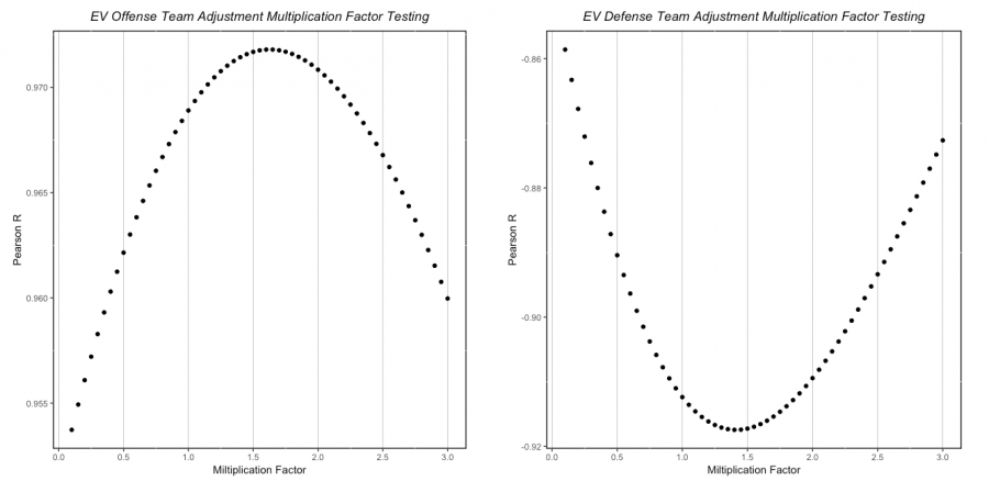
In order to adjust for team strength, we will use the same calculation that Myers laid out above; however, we will determine the multiplication value in a different manner. The multiplication value is determined by summing all players’ expanded above-average totals (for each of the four strength states) over the same timeframe that we used for the RAPM method and then finding the correlation with each player’s expanded respective RAPM coefficient (for each of the four strength states). This is looped over a range of values that start at 0.1 and increase by .05 up to 3.0 (10% up to 300% in the terms of Myers’ BPM adjustment). We then determine which multiplication factor results in the player summed values that most closely mirror the 11-year RAPM that the models were trained on.
Since we are using separate metrics for each of the components (GF for EV and PP offense and xGA for EV and SH defense), we will need to do this four times. Here is this process in visual form for even-strength and powerplay/shorthanded:
Even-Strength Team Adjustment Validation:

Powerplay / Shorthanded Team Adjustment Validation:

The multiplication factors determined from this process are as follows:
- EV Offense: 1.6 (160%)
- EV Defense: 1.4 (140%)
- PP Offense: 1.3 (130%)
- SH Defense 1.3 (130%)
With these we can now complete the team adjustment that will be applied to the raw SPM model outputs. We will use Jake Gardiner’s ‘17-18 season to demonstrate (EV offense). The calculation looks like this:
Per 60 adjustment value: ([1.6 * team_EV_GF60] – [SPM_EVO_AA_60 * TOI_perc_EV]) / team_skaters_EV
Total adjustment applied (per 60 adj / 60) * player EV TOI
Final “adjusted” EVO GAA: SPM_EVO_AA + total adj
For Jake Gardiner’s EV offense in ‘17-18, this looks like:
Per 60 adjustment value: ([1.6 * 0.263] – [-0.027 * 0.386]) / 4.96 = 0.087
Total adjustment applied (.087 / 60) * 1594.6 = 2.31
Final “adjusted” EVO GAA: -0.73 + 2.31 = 1.6
So, the original EVO GAA for Gardiner in this season was -0.73, but after applying the team adjustment he ends with a final value of 1.6 EVO GAA.
The process above is the same for each component with the team RAPM coefficients from the PP/SH centered around 0 (as these coefficients do not have 0 as their mean inherently). To get an idea of how this adjustment works overall, we can look at the total goals added to each player’s raw expanded SPM output (above average) compared to their respective team’s RAPM rating:
EV Offense:

EV Defense:

We see that the players with the most TOI who play on the worst/best teams in the league are impacted the most. Additionally, we can see that this effect is linear. The change here is somewhat minimal, but there is definitely room to further explore this adjustment/concept.
We’ve reached the end of our modeling processes! We’ve now laid out the “guts” of the RAPM and SPM models, which are the foundation for our WAR model. These together give us the basis for four of the five components of skater WAR (EV Offense, EV Defense, Powerplay Offense, Shorthanded Defense). The last remaining component is penalties – both drawn and taken. We will cover that in part 3 when we address replacement level and combining everything together among other topics.
Super Based guys thanks.